Beispiel-Projekte
In diesem Kapitel werden anhand der IoT-Szenarien und des IoT-Architekturmodells Übungs- und Umsetzungsbeispiele behandelt.
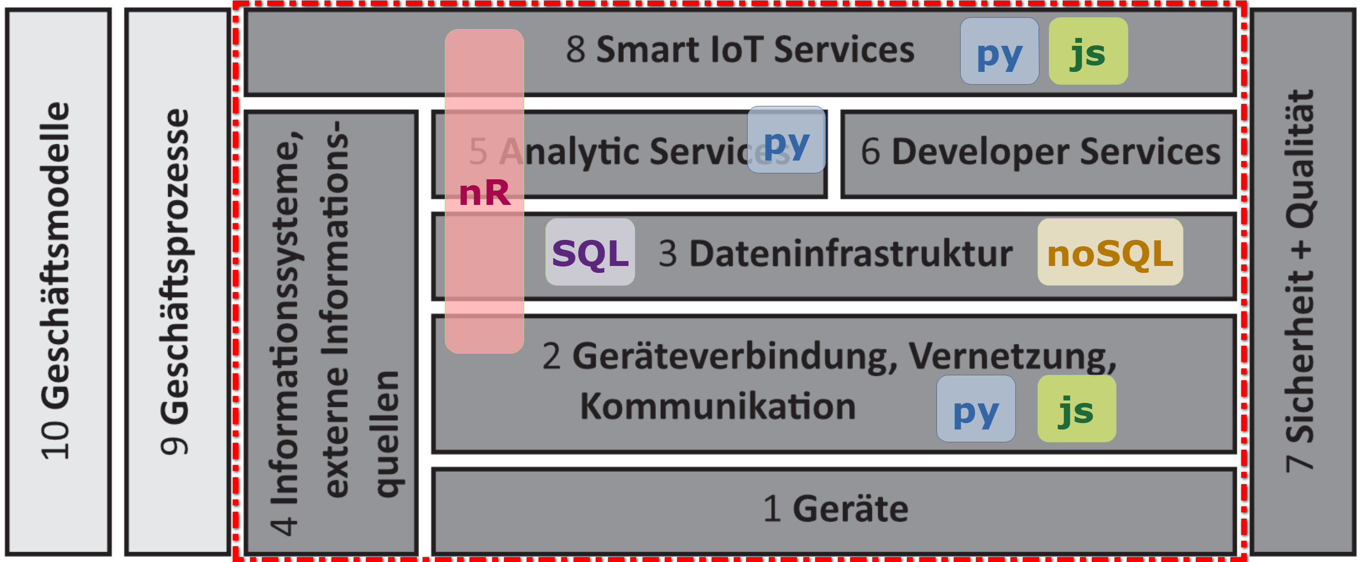
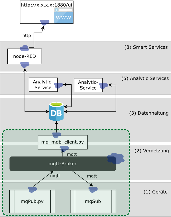
Sprachen für eine IoT-Plattform
Auf den rotumrandeten Bereich liegt der Fokus!
In der Regel werden die Projekte mit Hilfe einer Simulation umgesetzt. Diese kann in allen ebenen der IoT-Architektur eingreifen:
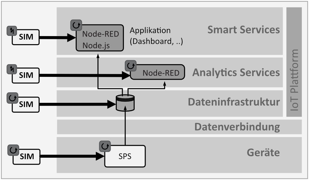
Allgemeines Konzept zur Einbindung von Simulationen entlang der IoT-Plattform-Architektur
Signale generieren mit Python
Erster Gehversuch mit VS Code und Python, um eine Datenquelle zur Verfügung zu haben.
# Bibliotheken importieren
import numpy as np
import time
…
# Parameter initialisieren
n = 10
x = np.zeros(n)

# Berechnungen
for i in range(n):
    x[i] = np.sin(i/1.23)


# Ausgabe
print(f’Ergebniss: {x}mm’)
Weitere Aufgaben:
- Rechteck-Generator
- PT1-Prozessverhalten (ideal)
-
- Stochastische Störungen
-
- Drift
- Random Walk
Skripte
| Datei | Link |
|---|---|
| squareSignal.py | File |
| sinusSignal.py | File |
| RandomWalk.py | File |
mqtt-nodeRED
Mit mqtt sollen hier Daten aus der Ebene (1) in die Ebene "Smart Services" (8) übertragen werden. Die Ereignisorientierung von mqtt kann untersucht werden.
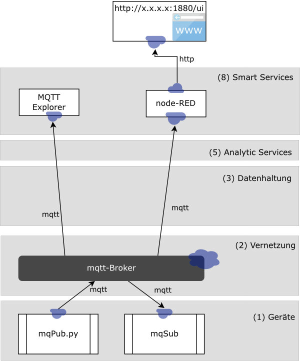
mqtt + Python + NodeRed
Software-Voraussetzungen
Info
| Software | Link |
|---|---|
| mqtt-Broker "Mosquitto" | Installation |
| mqtt-Explorer | Installation |
| Python | Installation |
| VS Code | Installation |
| NodeRed | Installation |
Aufgaben
- Publisher mit Python (
mqpub.py) - mqtt-Explorer ->
msg-Objectuntersuchen - Subscriber mit Python (
mqsub.py) - Node-Flow entwickeln
Skripte
Multi-Topics
'''
Einfacher Publisher
=============================
client.publish (sequentielles Publish) und
publish.multiple(msgs,...)
veröffentlichen jeweils "Einzel"-Topic, die vom Subscriper sequentiell empfangen werden

=> Dieses Skript setzt "subscriber_2.py" voraus

'''

import time

import paho.mqtt.client as mqtt
import paho.mqtt.publish as publish
import numpy as np

# --------------------------------------------------------------
# Parameterblock
mq_host = "127.0.0.1"        # lokaler PC
# mq_host = "172.18.45.150"    # Labor-Server
mq_topic = "test_172"   # letzte IP-Adr-Nr

# --------------------------------------------------------------

def on_connect(client, userdata, flags, rc):
    print("Connected with result code " + str(rc))


client = mqtt.Client()
client.on_connect = on_connect

client.connect(mq_host, 1883, 60)

client.loop_start()

t = 0.0
while True:
    time.sleep(2)
    t = t + 0.01
#     client.publish(f"{mq_topic}/temperature", t)
#     client.publish(f"{mq_topic}/sinus", np.sin(t))
    msgs = [(f"{mq_topic}/cos",np.cos(t)),
            (f"{mq_topic}/cos2",np.cos(t)*2),
            (f"{mq_topic}/ts",time.time())]
    publish.multiple(msgs, hostname=mq_host)
    print(msgs)
'''
Einfacher Abonnent
======================
mit jedem abonnierten Topic wird die on_message-funktion aufgerufen
(globaler Zähler cnt)

Dieses Skript setzt den Publisher "sensor_multiple_2.py" voraus

https://pypi.org/project/paho-mqtt/#description
'''
import paho.mqtt.client as mqtt

# --------------------------------------------------------------
# Parameterblock
mq_host = "127.0.0.1"        # lokaler PC
# mq_host = "172.18.45.150"    # Labor-Server
mq_topic = "test_172"   # letzte IP-Adr-Nr

# --------------------------------------------------------------


cnt = 0

def on_connect(client, userdata, flags, rc):
    print("Connected with result code " + str(rc))

    client.subscribe(mq_topic+"/#")

def on_message(client, userdata, msg):
    global cnt
    cnt +=1
    print(cnt, '     ',msg.topic + " " + str(msg.payload))


client = mqtt.Client()
client.on_connect = on_connect
client.on_message = on_message

client.connect(mq_host, 1883, 60)

client.loop_forever()
json-Objects
'''
JSON-Publisher
=============================
client.publish (sequentielles Publish) und
publish.multiple(msgs,...)
veröffentlicht ein "Sammel"-Topic mit client.publish(), das vom Subscriper
als JSON-Objekt empfangen wird.

=> Dieses Skript setzt "subscriber_3_json.py"  oder
   "subscriber_3_json_mDB_2.py" voraus

'''


import time

import paho.mqtt.client as mqtt
import paho.mqtt.publish as publish
import numpy as np
import json

def on_connect(client, userdata, flags, rc):
    print("Connected with result code " + str(rc))

# Parameterblock
mq_host = "127.0.0.1"        # lokaler PC
# mq_host = "172.18.45.150"    # Labor-Server
mq_topic = "test_172"   # letzte IP-Adr-Nr

client = mqtt.Client()
client.on_connect = on_connect

client.connect(mq_host, 1883, 60)

client.loop_start()

t = 0.0
while True:
    time.sleep(1)
    t = t + 0.01
    # python-dict beschreibt den Daten-Block (payload)
    PL = {"cos":np.cos(t),
        "cos2":np.cos(t)*2,
        "ts":time.time()
        }
    # Umwandeln in ein json-Objekt
    jPL = json.dumps(PL)
    # versenden (publish)
    client.publish(topic=mq_topic, payload = jPL)
    print(jPL)
#!/usr/bin/env python

'''
https://pypi.org/project/paho-mqtt/#description
'''
import paho.mqtt.client as mqtt
import json

cnt = 0

def on_connect(client, userdata, flags, rc):
    print("Connected with result code " + str(rc))

    client.subscribe("sen/#")
    client.subscribe("test_172")

def on_message(client, userdata, msg):
    global cnt
    cnt +=1
    # print(cnt, '     ',msg.topic + " " + str(msg.payload))
    data = json.loads(msg.payload)
    # print(cnt, '     ',data)
    print(cnt, '     ',data["ts"])


client = mqtt.Client()
client.on_connect = on_connect
client.on_message = on_message

client.connect("localhost", 1883, 60)

client.loop_forever()
subscriber_3_json.py
mqtt-NodeRED-MongoDB
Durch die Schicht (3) Datenhaltung lassen sich auch Historie-Daten für Analysezwecke nutzen.
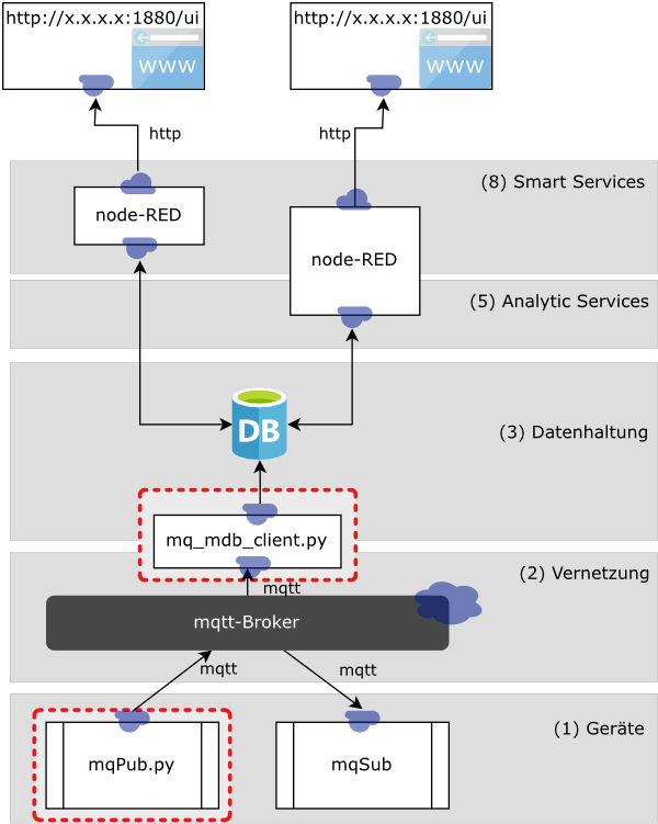
mqtt + Python + MongoDB + NodeRed
Software-Voraussetzungen
Info
| Software | Link |
|---|---|
| Mongo-DB (inkl. Compass) | Installation |
Aufgaben
mq_mdb_client.py->PY-sim_mqtt_mdb_NR/subscriber_3_json_mDB_2.pyanpassen und startensensor_json_3.py->PY-sim_mqtt_mdb_NR/sensor_json_3_2.pyanpassen und separat starten (Konsole, ...)- mdb-Explorer auf mDB setzen
- NodeRed-Flows mit mDB-Verbindungen entwickeln
Skripte
pub / sub
'''
IoT-Schicht 1
- Publishd mqtt-basierte Daten (simulierter Prozess)

letzte Änderung: 27.4.2023

Doku:
https://pypi.org/project/paho-mqtt/#description
'''

import time

import paho.mqtt.client as mqtt
import numpy as np
import json
import datetime
# --------------------------------------------------------------
# Parameterblock
mq_host = "127.0.0.1"        # lokaler PC
# mq_host = "172.18.45.150"    # Labor-Server
mq_topic = "test_172"   # letzte IP-Adr-Nr

# --------------------------------------------------------------


def on_connect(client, userdata, flags, rc):
    print("Connected with result code " + str(rc))


# __main__ ======================================================
client = mqtt.Client()
client.on_connect = on_connect

client.connect(mq_host, 1883, 60)

client.loop_start()

# Generieren von simulierten Daten -----------
cnt = 0
while True:
    time.sleep(1)
    cnt += 10
    ts = datetime.datetime.now()
    # python-dict beschreibt den Daten-Block (payload)
    PL = {"t": time.time(),     # unix-Zeit
        "ts": str(ts),          # utf-Zeit
        "cnt": cnt,
        "v1": np.random.normal(),
        "v2":np.cos(cnt/10)*2,
        "v3": np.cos(cnt/20)*200
        }
    # Umwandeln in ein json-Objekt
    jPL = json.dumps(PL)
    # versenden (publish)
    client.publish(topic=mq_topic, payload = jPL )
    print(PL)
'''
IoT-Schicht 2-3
- subribed mqtt-basierte json-Daten
- schreibt die Daten in die MongoDB

=> setzt das Skript "sensor_json_3.py" voraus (schreibt als payload ein json-Objekt).


letzte Änderung: 27.4.2023

Doku:
https://pypi.org/project/paho-mqtt/#description
https://pymongo.readthedocs.io/en/stable/
'''
import paho.mqtt.client as mqtt
from pymongo import MongoClient
import json
# --------------------------------------------------------------
# Parameterblock
mdb_mq_host = "127.0.0.1"        # lokaler PC
# mdb_mq_host = "172.18.45.150"    # Labor-Server
mdb_db = "test"
mdb_col = "M_172"       # letzte IP-Adr-Nr
mq_topic = "test_172"   # letzte IP-Adr-Nr

# --------------------------------------------------------------

cnt = 0

class mqClient():
    def __init__(self,col):
        self.col = col

    def on_connect(self,client, userdata, flags, rc):
        print("Connected with result code " + str(rc))
        client.subscribe("test_172")

    def on_message(self,client, userdata, msg):
        global cnt
        cnt +=1
        print(cnt, '     ',msg.topic + " " + str(msg.payload))
        # payload enthält ein json-Objekt mit allen gesendeten Datenwerten {key1:value1, key2:value2}
        data = json.loads(msg.payload)
        print(data)
        # Schreiben in die MongoDB
        result = self.col.insert_one(data)

# __main__ ======================================================
mo_client = MongoClient(mdb_mq_host, 27017)
db = mo_client[mdb_db]
col = db[mdb_col]
# col.drop()      # Löschen der bereits erzeugten Collection (ggf. auskommentieren...)

mqC = mqClient(col)

client = mqtt.Client()
client.on_connect = mqC.on_connect
client.on_message = mqC.on_message

client.connect(mdb_mq_host, 1883, 60)

client.loop_forever()
NodeRed
Für den Zugriff auf die MongoDB in NodeRed muss das Node-Paket "node-red-contrib-mongodb4" installiert sein.
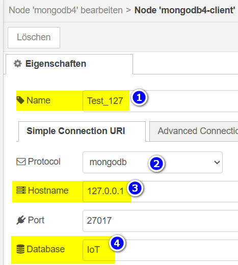
Konfiguration der MongoDB-Schnittstelle
Die eigentliche Suche (query) wird mit dem Node-Parameterdialog (2-4) eingestellt:
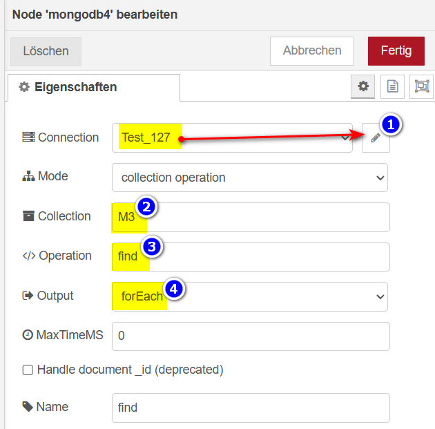
Konfiguration des MongoDB-Node
Als Input auf den MongoDB-Node liefert der Function-Node die eigentliche Such-Anfrage (hier: limit = 2 !!):
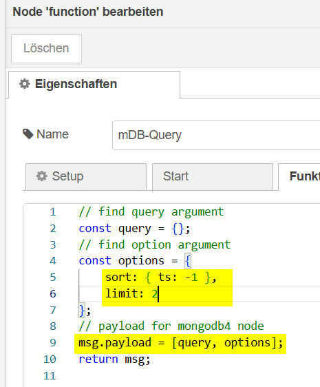
Function-Node
Javascript
// find query argument
const query = {};
// find option argument
const options = {
    sort: { ts: -1 },
    limit: 2
};
// payload for mongodb4 node
msg.payload = [query, options];
return msg;
Damit liefert die Abfrage 2 "Documents" zurück:
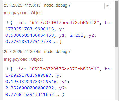
Result der Abfrage
flows_contribMDB.json
[
{
    "id": "36ac58d44b0a6fbb",
    "type": "tab",
    "label": "Flow 2",
    "disabled": false,
    "info": "",
    "env": []
},
{
    "id": "f4334596e259510e",
    "type": "inject",
    "z": "36ac58d44b0a6fbb",
    "name": "",
    "props": [
        {
            "p": "payload"
        },
        {
            "p": "topic",
            "vt": "str"
        }
    ],
    "repeat": "",
    "crontab": "",
    "once": false,
    "onceDelay": 0.1,
    "topic": "",
    "payload": "",
    "payloadType": "date",
    "x": 180,
    "y": 180,
    "wires": [
        [
            "248a30f8569a9831"
        ]
    ]
},
{
    "id": "248a30f8569a9831",
    "type": "function",
    "z": "36ac58d44b0a6fbb",
    "name": "mDB-Query",
    "func": "// find query argument\nconst query = {};\n// find option argument\nconst options = {\n    sort: { ts: -1 },\n    limit: 2\n};\n// payload for mongodb4 node\nmsg.payload = [query, options];\nreturn msg;\n",
    "outputs": 1,
    "timeout": 0,
    "noerr": 0,
    "initialize": "",
    "finalize": "",
    "libs": [],
    "x": 350,
    "y": 180,
    "wires": [
        [
            "9f451ce54d300234"
        ]
    ]
},
{
    "id": "9f451ce54d300234",
    "type": "mongodb4",
    "z": "36ac58d44b0a6fbb",
    "clientNode": "ceb5e2fe4fbc5cac",
    "mode": "collection",
    "collection": "M3",
    "operation": "find",
    "output": "forEach",
    "maxTimeMS": "0",
    "handleDocId": false,
    "name": "find",
    "x": 510,
    "y": 180,
    "wires": [
        [
            "b455d65d1ab4bd1d",
            "7fda93745a6cc2dc"
        ]
    ]
},
{
    "id": "b455d65d1ab4bd1d",
    "type": "debug",
    "z": "36ac58d44b0a6fbb",
    "name": "debug 10",
    "active": true,
    "tosidebar": true,
    "console": false,
    "tostatus": false,
    "complete": "true",
    "targetType": "full",
    "statusVal": "",
    "statusType": "auto",
    "x": 700,
    "y": 180,
    "wires": []
},
{
    "id": "7fda93745a6cc2dc",
    "type": "function",
    "z": "36ac58d44b0a6fbb",
    "name": "function 4",
    "func": "msg.payload = msg.payload.y;\nreturn msg;",
    "outputs": 1,
    "timeout": 0,
    "noerr": 0,
    "initialize": "",
    "finalize": "",
    "libs": [],
    "x": 660,
    "y": 300,
    "wires": [
        [
            "32d6ada36d21c1f6"
        ]
    ]
},
{
    "id": "32d6ada36d21c1f6",
    "type": "debug",
    "z": "36ac58d44b0a6fbb",
    "name": "debug 11",
    "active": false,
    "tosidebar": true,
    "console": false,
    "tostatus": false,
    "complete": "true",
    "targetType": "full",
    "statusVal": "",
    "statusType": "auto",
    "x": 820,
    "y": 300,
    "wires": []
},
{
    "id": "ceb5e2fe4fbc5cac",
    "type": "mongodb4-client",
    "name": "Test_127",
    "protocol": "mongodb",
    "hostname": "127.0.0.1",
    "port": "27017",
    "dbName": "IoT",
    "appName": "",
    "authSource": "",
    "authMechanism": "DEFAULT",
    "tls": false,
    "tlsCAFile": "",
    "tlsCertificateKeyFile": "",
    "tlsInsecure": false,
    "connectTimeoutMS": "",
    "socketTimeoutMS": "",
    "minPoolSize": "",
    "maxPoolSize": "",
    "maxIdleTimeMS": "",
    "uri": "",
    "advanced": "",
    "uriTabActive": "tab-uri-simple"
}
]
mqtt-py3-MongoDB-NR
In der nächsten Stufe soll die Analytic Services dazukommen. Die Schichten 1 bis 3 wurden bereits vollständig umgesetzt. Wird nun der Fokus im Entwicklungsprozess auf die Prozess-Simulation in Anlehnung an den realen Prozess gerichtet, dann können die simulierten Prozessdaten hierzu direkt in die Datenbank geschrieben werden (Grün markierter Bereich 1,2 +3).
mqtt + Python + MongoDB + pyAnalytics + NodeRed
Diese Variante zeigt das Skript
client
| PY-simProz_mDB_NR\sim__mdb_prozSig_rt_02.py | |
|---|---|
1 2 3 4 5 6 7 8 9 10 11 12 13 14 15 16 17 18 19 20 21 22 23 24 25 26 27 28 29 30 31 32 33 34 35 36 37 38 39 40 41 42 43 44 45 46 47 48 49 50 51 52 53 54 55 56 57 58 59 60 61 62 63 64 65 66 67 68 69 70 71 72 73 74 75 76 77 78 79 80 81 82 83 84 85 86 87 88 89 90 91 92 93 94 95 96 97 98 99 100 101 102 103 104 105 106 | |
Download (PT1-Filter): File
In diesem Python-Skript werden mehrere simulationsspezifische Teillösungen verwendet:
Steuerung der Simulation
Dieser Simulation basiert auf der Idee, dass die Simulation in zwei zeitlich aufeinander folgende Phasen aufgeteilt wird:
- Berechnung und Speicherung von Prozessdaten "as quick as possible": Dieser Vorlauf generiert historische Datensätze mit
tsA = tsE - pd.Timedelta(1,"h")(Zeile 90)(hier 1 Stunde) - Ist der Zeitpunkt
now()erreicht, läuft die Simulation in Echtzeit mit der Abtastzeitts = ts + pd.Timedelta(dT,T_unit)(Zeile 97) weiter, bis das Skript mit Ctrl+C abgebrochen wird.
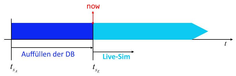
Zwei Phasen der Simulation
| Ausschnitt: Phase 1+2 | |
|---|---|
1 2 3 4 5 6 7 8 9 10 11 12 13 14 15 16 17 18 | |
- Tranfer in MongoDB mit berechnetem Timestamp
ts - Tranfer in MongoDB mit "echtem" Timestamp
pd.Timestamp.now()in functionwrite_mdb_now()
Info
Folgende Anpassungen müssen vorgenommen werden:
- MongoDB: IP & Port (
client = MongoClient('localhost', 27017)) - MongoDB: Datenbank (
db = client['IoT']) - MongoDB: Collection (
col = db["m"]) - Simulationsvorlauf:
tsA = tsE - pd.Timedelta(1,"h")
Analytic-Services
Die Analytic-Services (Datenanalyse-Prozesse) wurden in den vorangegangen Beispielen in NodeRed realisiert. Um sie als SmartServices umzusetzen, sollen sie nun als eigenständige Python-Programme realisiert werden.
Aufgabe 1: Zyklische Analyse
Die erste Aufgabe besteht in der zyklischen Berechunng statistischer Kennwerte einer Zeitreihe. Der Simulationsprozess liefert das Signal \(u(t)\). Die Berechnung des Mittelwertes:
und der Standardabweichung
lassen sich mit Hilfe der Methoden mean() und std() eines pandas-Dataframes berechnen:
#  Analyse-Operationen
uMean = u.mean()
uStd = u.std()
errCnt = err.sum()
Die Methode sum()berechnet die Summe der Fehler-Ereignisse.
Datenflow
Die Datenverarbeitung dieses Analyseprozesses läuft in drei Schritten ab:
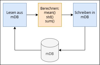
Zyklische Analyse
Für den zyklischen Prozess wird hier wieder das Pakage APScheduler eingesetzt APScheduler
Konfiguration
Hier wird die Konfiguration, wie IP-Adresse, Datenbank und Collection etc. durch die toml-Datei cfg.tomlvorgenommen:
Toml
| PY-simProz_mDB_NR\cfg.toml | |
|---|---|
1 2 3 4 5 6 7 8 9 10 11 12 13 14 15 16 17 | |
Gesamt-Script
Python Analytic
| PY-simProz_mDB_NR\analytic_mDB_02.py | |
|---|---|
1 2 3 4 5 6 7 8 9 10 11 12 13 14 15 16 17 18 19 20 21 22 23 24 25 26 27 28 29 30 31 32 33 34 35 36 37 38 39 40 41 42 43 44 45 46 47 48 49 50 51 52 53 54 55 56 57 58 59 60 61 62 63 64 65 66 67 68 69 70 71 72 73 74 75 76 77 78 79 80 81 82 83 84 85 86 87 88 89 90 | |
- Event-Ereigniss
- MongoDB-Abfrage auf das Zeitfenster t_sA > t > t_sE
- Speichern in der MongoDB
- Für Entwicklungszwecke !!
- Erzeugen des Schedulers
- Starten des zyklischen Analytic-Jobs
Download: File
Aufgabe 2: Erweiterung der zyklische Analyse
Wenn die Analyseergebnisse automatisiert durch einen weiteren Prozesse (Node-Red, Python, ...) weiterverarbeitet werden sollen, dann kann z.B. das Ereigniss "Analyse-Ergebniss liegt vor, mittels einem "Mqtt-Publish" anderen "Subscribern" zur Verfügung gestellt werden.
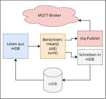
Zyklische Analyse
Dem Analytic-Service analytic_mDB_mq_01.py wird die Klasse clMqttConn hinzugefügt:
Python Analytic + Mqtt
| PY-simProz_mDB_NR\analytic_mDB_mq_01.py | |
|---|---|
1 2 3 4 5 6 7 8 9 10 11 12 13 14 15 16 17 18 19 20 21 22 23 24 25 26 27 28 29 30 31 32 33 34 35 36 37 38 39 40 41 42 43 44 45 46 47 48 49 50 51 52 53 54 55 56 57 58 59 60 61 62 63 64 65 66 67 68 69 70 71 72 73 74 75 76 77 78 79 80 81 82 83 84 85 86 87 88 89 90 91 92 93 94 95 96 97 98 99 100 101 102 103 104 105 106 107 108 109 110 111 112 113 114 115 116 117 118 119 120 121 122 123 124 125 126 127 128 129 | |
Download: File
Dashboard-Service
In der Abbildung ist ein NodeRed-Visualisierug vorgesehen. Diese kann wie bereits gezeigt den Datenbankzugriff auf die MongoDB vornehmen und die Dahboard-Widgets bereitstellen. Alternativ soll hier in einem zweiten Schritt eine Lösung mittels Proxy-Server aufgezeigt werden.
Node-Red (Visu u. mDB)
Node-Red-Visu und py-Proxy
Aufteilung und Systematisierung der Frontend- und Backend-Entwicklung.
Backend: Python - FastApi
Datenbank-Zugriffe und Analytic Services lassen sich deutlich besser in Python umsetzen. Die Schnittstelle zu Node-Red kann entweder über Message-Routine via MQTT oder Endpoints einer RestApi realisiert werden. Beide Varianten lassen sich sehr einfach realisieren und gut debuggen.
RestApi mit FastApi
Rumpf-Skript:
Python Backend
| py_nr/fapi_1.py | |
|---|---|
1 2 3 4 5 6 7 8 9 10 11 12 13 14 15 16 17 18 19 20 21 22 | |
- Webserver (muss vorher installiert worden sein uvicorn)
- Root-Endpoint (zum Testen)
- Endpoint für NodeRed-http-request
- Webservice starten mit uvicorn
Getestet werden der Server mit Hilfe des Tools curl(1):
curlist ein Konndozeilen-Tool, dass unterschiedlichste Protokolle beherrscht. Link
curl 127.0.0.1:8001/sfcn -X POST
In Node-Red werden der Node "http request" eingesetzt:
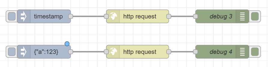
Der erste Request zeigt einen einfache Get-Aufruf:
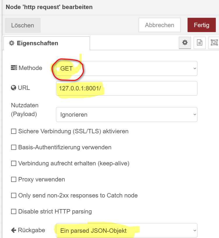
Er zeigt direkt auf den root-Endpoint, der das Message-json-Objekt {"message": "Hello World"} zurückliefert.
Der zweite Request demonstriert einen Post-Request. Der NR-Client sendet hier ein json-Objekt an den Server. Dieser antwortet ebenfalls mit einem json-Objekt:
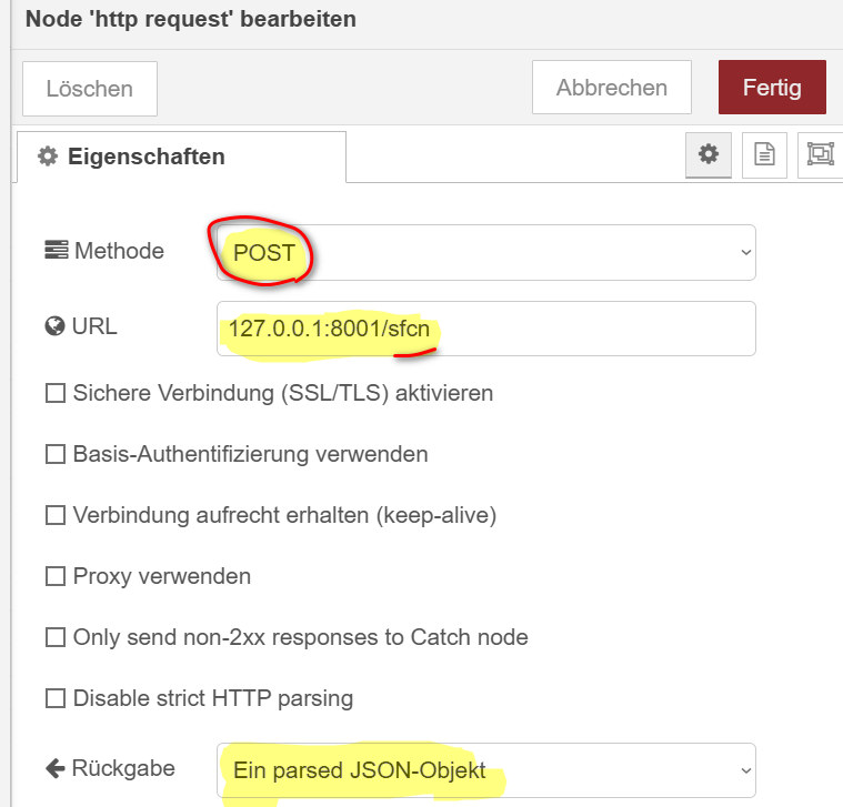
Er zeigt auf den Endpoint @app.post("/sfcn"), der das Message-json-Objekt {"payload": {"sin": 12.34, "cos":0.231}} zurückliefert.
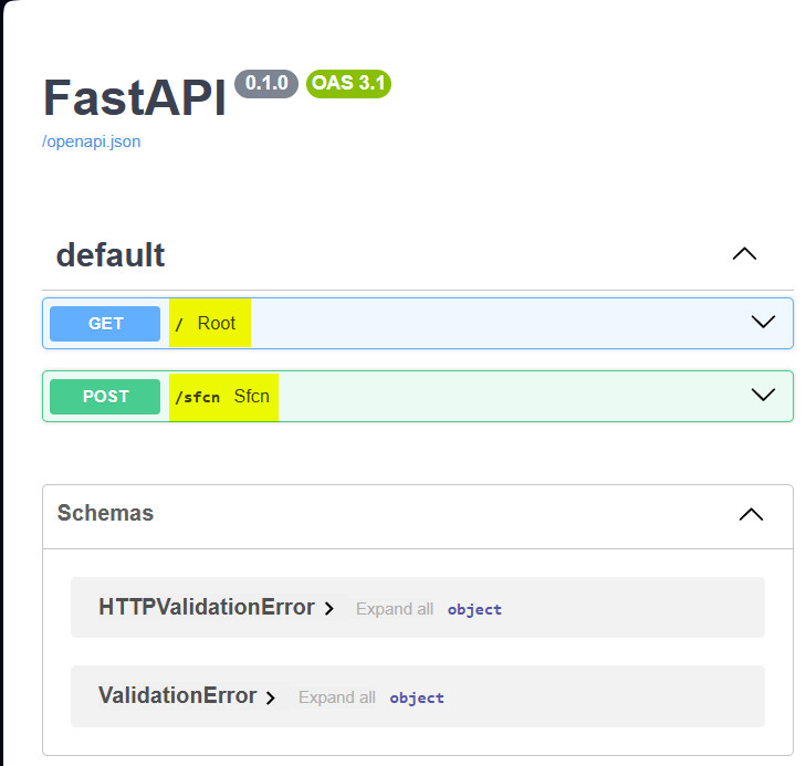
Der große Vorteil von FastApi ist die Möglichkeit, die API-Schnittstelle automatisch zu dokumentieren und testen zu können:
127.0.0.:8001/docs
Wird ein Post-Request abgesetzt,
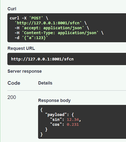
Dann erhält man direkt das json-Objekt der Antwort.